The Geek’s Guide to ML Experimentation

Table of Links

Abstract and 1. Introduction

1.1 Post Hoc Explanation

1.2 The Disagreement Problem

1.3 Encouraging Explanation Consensus

1. Related Work

2. Pear: Post HOC Explainer Agreement Regularizer

3. The Efficacy of Consensus Training

   4.1 Agreement Metrics

   4.2 Improving Consensus Metrics

   [4.3 Consistency At What Cost?]()

   4.4 Are the Explanations Still Valuable?

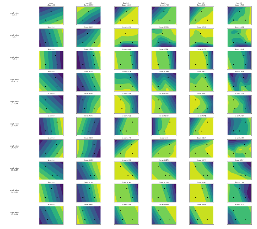
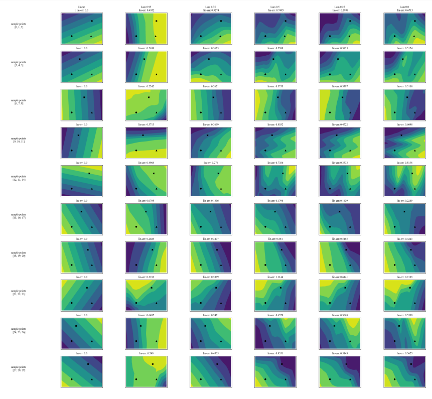
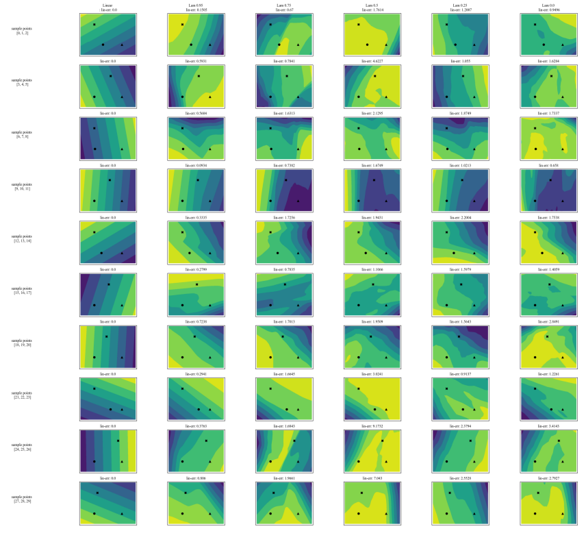
   4.5 Consensus and Linearity

   4.6 Two Loss Terms

4. Discussion

   5.1 Future Work

   5.2 Conclusion, Acknowledgements, and References

Appendix

A APPENDIX

A.1 Datasets

In our experiments we use tabular datasets originally from OpenML and compiled into a set of benchmark datasets from the Inria-Soda team on HuggingFace [11]. We provide some details about each dataset:

\ Bank Marketing This is a binary classification dataset with six input features and is approximately class balanced. We train on 7,933 training samples and test on the remaining 2,645 samples.

\ California Housing This is a binary classification dataset with seven input features and is approximately class balanced. We train on 15,475 training samples and test on the remaining 5,159 samples.

\ Electricity This is a binary classification dataset with seven input features and is approximately class balanced. We train on 28,855 training samples and test on the remaining 9,619 samples.

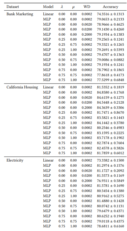
A.2 Hyperparameters

Many of our hyperparameters are constant across all of our experiments. For example, all MLPs are trained with a batch size of 64, and initial learning rate of 0.0005. Also, all the MLPs we study are 3 hidden layers of 100 neurons each. We always use the AdamW optimizer [19]. The number of epochs varies from case to case. For all three datasets, we train for 30 epochs when 𝜆 ∈ {0.0, 0.25} and 50 epochs otherwise. When training linear models, we use 10 epochs and an initial learning rate of 0.1.

A.3 Disagreement Metrics

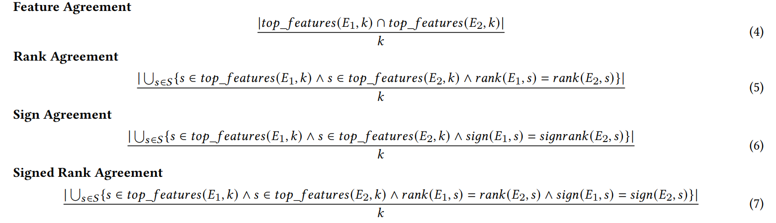
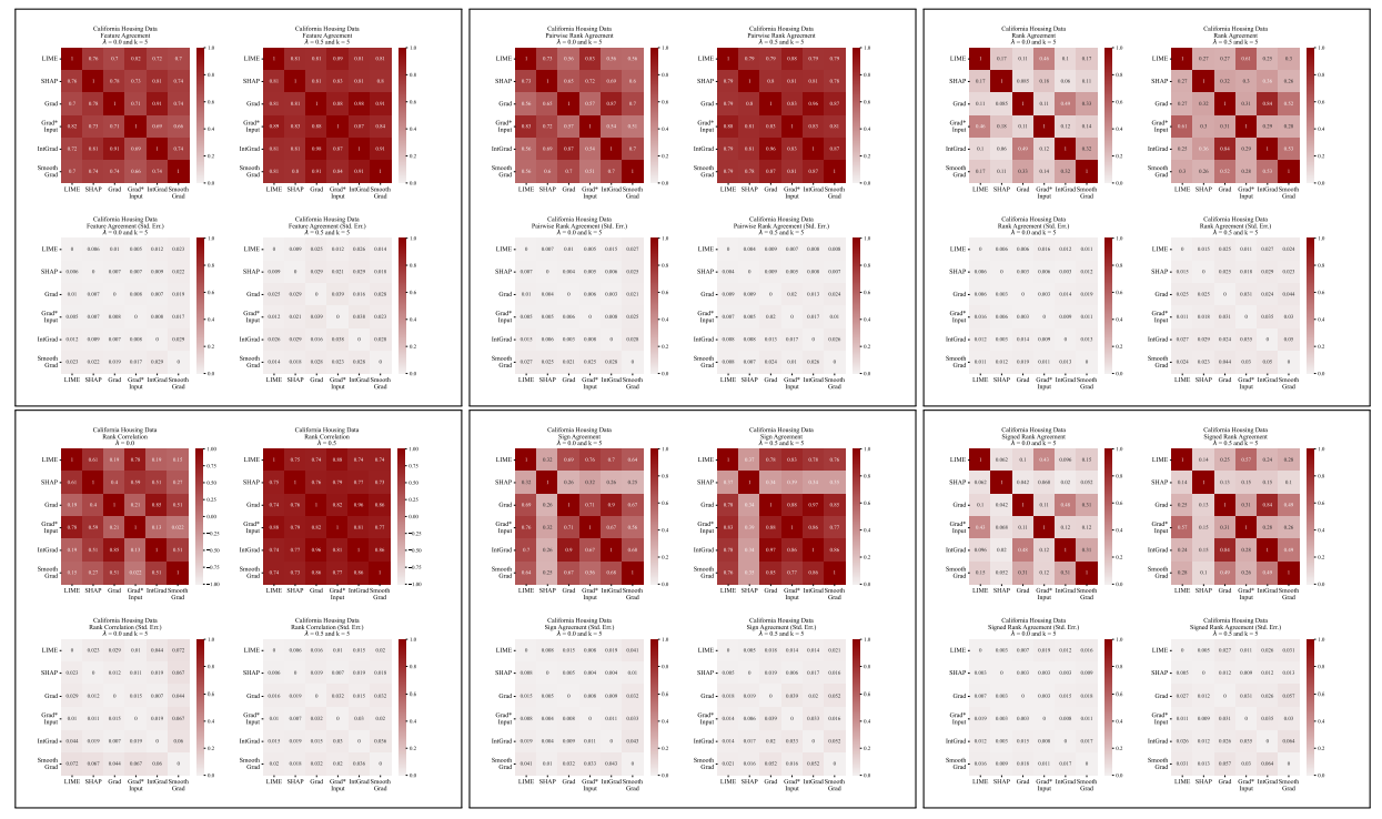
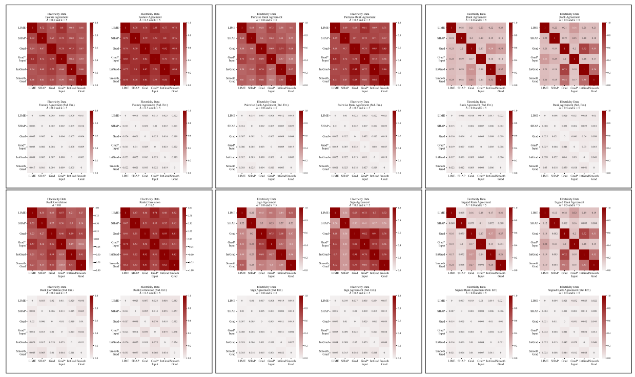
We define each of the six agreement metrics used in our work here.

\ The first four metrics depend on the top-𝑘 most important features in each explanation. Let 𝑡𝑜𝑝_𝑓 𝑒𝑎𝑡𝑢𝑟𝑒𝑠(𝐸, 𝑘) represent the top-𝑘 most important features in an explanation 𝐸, let 𝑟𝑎𝑛𝑘 (𝐸, 𝑠) be the importance rank of the feature 𝑠 within explanation 𝐸, and let 𝑠𝑖𝑔𝑛(𝐸, 𝑠) be the sign (positive, negative, or zero) of the importance score of feature 𝑠 in explanation 𝐸.

\

\ The next two agreement metrics depend on all features within each explanation, not just the top-𝑘. Let 𝑅 be a function that computes the ranking of features within an explanation by importance.

\

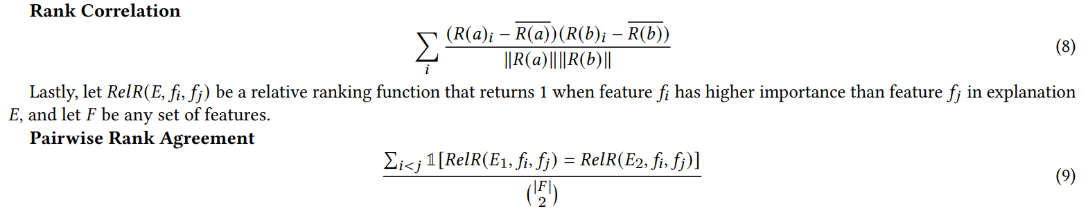
\ (Note: Krishna et al. [15] specify in their paper that 𝐹 is to be a set of features specified by an end user, but in our experiments we use all features with this metric).

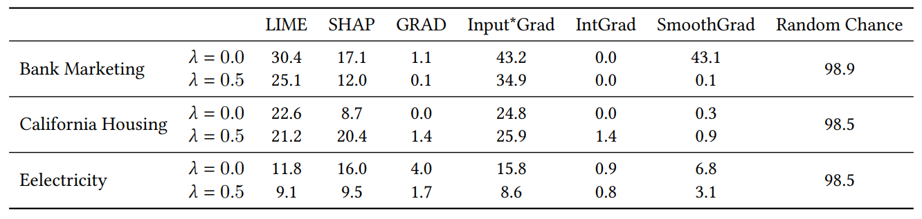
A.4 Junk Feature Experiment Results

When we add random features for the experiment in Section 4.4, we double the number of features. We do this to check whether our consensus loss damages explanation quality by placing irrelevant features in the top-𝐾 more often than models trained naturally. In Table 1, we report the percentage of the time that each explainer included one of the random features in the top-5 most important features. We observe that across the board, we do not see a systematic increase of these percentages between 𝜆 = 0.0 (a baseline MLP without our consensus loss) and 𝜆 = 0.5 (an MLP trained with our consensus loss)

\

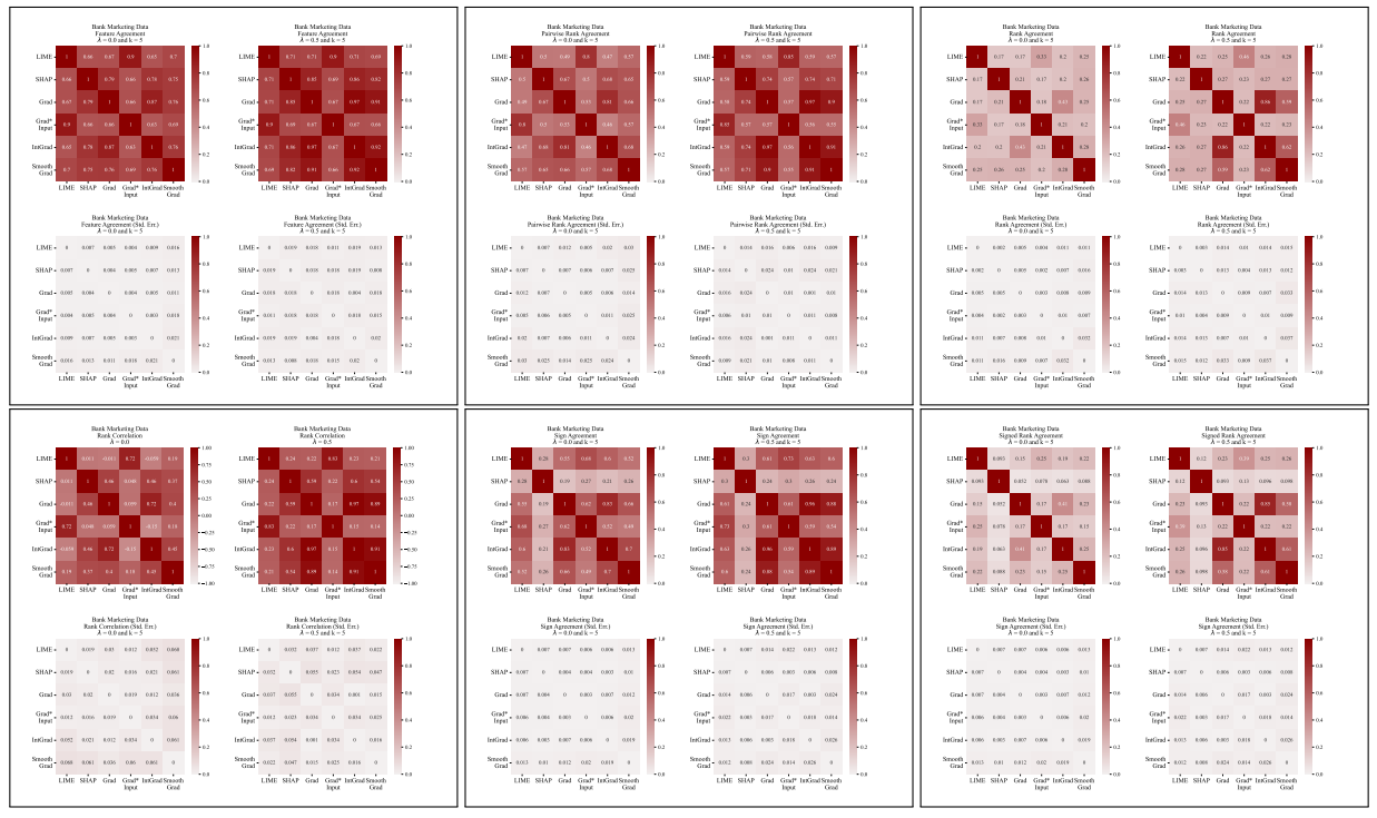
A.5 More Disagreement Matrices

\

\

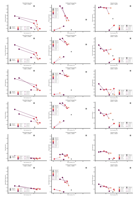
A.6 Extended Results

A.7 Additional Plots

\

\

\

\

:::info Authors:

(1) Avi Schwarzschild, University of Maryland, College Park, Maryland, USA and Work completed while working at Arthur (avi1umd.edu);

(2) Max Cembalest, Arthur, New York City, New York, USA;

(3) Karthik Rao, Arthur, New York City, New York, USA;

(4) Keegan Hines, Arthur, New York City, New York, USA;

(5) John Dickerson†, Arthur, New York City, New York, USA ([e-mail]).

:::

---

:::info This paper is available on arxiv under CC BY 4.0 DEED license.

:::

\